Least Square Method
Least square method is the process of finding a regression line or best-fitted line for any data set that is described by an equation. This method requires reducing the sum of the squares of the residual parts of the points from the curve or line and the trend of outcomes is found quantitatively. The method of curve fitting is seen while regression analysis and the fitting equations to derive the curve is the least square method.
Let us look at a simple example, Ms. Dolma said in the class "Hey students who spend more time on their assignments are getting better grades". A student wants to estimate his grade for spending 2.3 hours on an assignment. Through the magic of the least-squares method, it is possible to determine the predictive model that will help him estimate the grades far more accurately. This method is much simpler because it requires nothing more than some data and maybe a calculator.
In this section, we’re going to explore least squares, understand what it means, learn the general formula, steps to plot it on a graph, know what are its limitations, and see what tricks we can use with least squares.
| 1. | Least Square Method Definition |
| 2. | Limitations for Least Square Method |
| 3. | Least Square Method Graph |
| 4. | Least Square Method Formula |
| 5. | FAQs on Least Square Method |
Least Square Method Definition
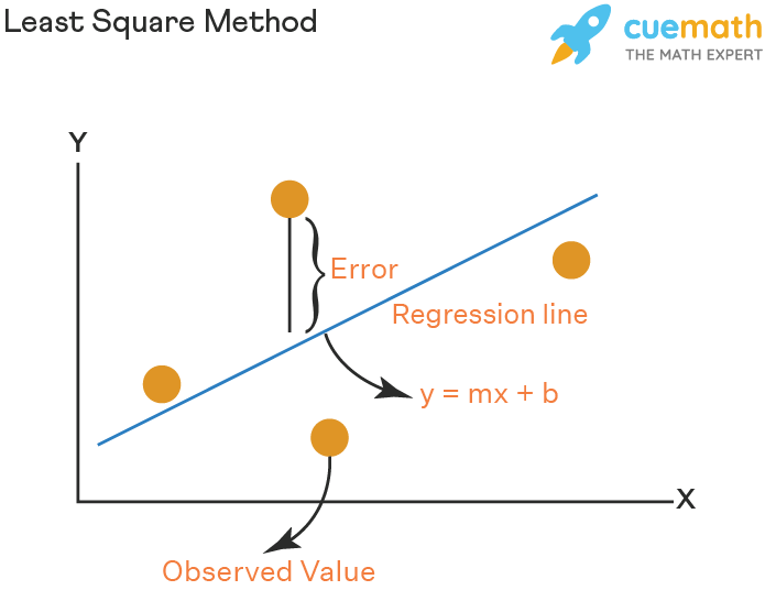
The least-squares method is a statistical method used to find the line of best fit of the form of an equation such as y = mx + b to the given data. The curve of the equation is called the regression line. Our main objective in this method is to reduce the sum of the squares of errors as much as possible. This is the reason this method is called the least-squares method. This method is often used in data fitting where the best fit result is assumed to reduce the sum of squared errors that is considered to be the difference between the observed values and corresponding fitted value. The sum of squared errors helps in finding the variation in observed data. For example, we have 4 data points and using this method we arrive at the following graph.

The two basic categories of least-square problems are ordinary or linear least squares and nonlinear least squares.
Limitations for Least Square Method
Even though the least-squares method is considered the best method to find the line of best fit, it has a few limitations. They are:
- This method exhibits only the relationship between the two variables. All other causes and effects are not taken into consideration.
- This method is unreliable when data is not evenly distributed.
- This method is very sensitive to outliers. In fact, this can skew the results of the least-squares analysis.
Least Square Method Graph
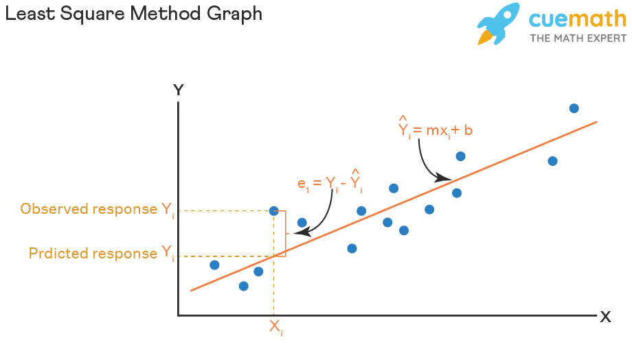
Look at the graph below, the straight line shows the potential relationship between the independent variable and the dependent variable. The ultimate goal of this method is to reduce this difference between the observed response and the response predicted by the regression line. Less residual means that the model fits better. The data points need to be minimized by the method of reducing residuals of each point from the line. There are vertical residuals and perpendicular residuals. Vertical is mostly used in polynomials and hyperplane problems while perpendicular is used in general as seen in the image below.

Least Square Method Formula
Least-square method is the curve that best fits a set of observations with a minimum sum of squared residuals or errors. Let us assume that the given points of data are (x1, y1), (x2, y2), (x3, y3), …, (xn, yn) in which all x’s are independent variables, while all y’s are dependent ones. This method is used to find a linear line of the form y = mx + b, where y and x are variables, m is the slope, and b is the y-intercept. The formula to calculate slope m and the value of b is given by:
m = (n∑xy - ∑y∑x)/[n∑x2 - (∑x)2]
b = (∑y - m∑x)/n
Here, n is the number of data points.
Following are the steps to calculate the least square using the above formulas.
- Step 1: Draw a table with 4 columns where the first two columns are for x and y points.
- Step 2: In the next two columns, find xy and (x)2.
- Step 3: Find ∑x, ∑y, ∑xy, and ∑(x)2.
- Step 4: Find the value of slope m using the above formula.
- Step 5: Calculate the value of b using the above formula.
- Step 6: Substitute the value of m and b in the equation y = mx + b
Let us look at an example to understand this better.
Example: Let's say we have data as shown below.
| x | 1 | 2 | 3 | 4 | 5 |
|---|---|---|---|---|---|
| y | 2 | 5 | 3 | 8 | 7 |
Solution: We will follow the steps to find the linear line.
| x | y | xy | x2 |
|---|---|---|---|
| 1 | 2 | 2 | 1 |
| 2 | 5 | 10 | 4 |
| 3 | 3 | 9 | 9 |
| 4 | 8 | 32 | 16 |
| 5 | 7 | 35 | 25 |
| ∑x =15 | ∑y = 25 | ∑xy = 88 | ∑x2 = 55 |
Find the value of m by using the formula,
m = (n∑xy - ∑y∑x)/[n∑x2 - (∑x)2]
m = [(5×88) - (15×25)]/[(5×55) - (15)2]
m = (440 - 375)/(275 - 225)
m = 65/50 = 13/10
Find the value of b by using the formula,
b = (∑y - m∑x)/n
b = (25 - 1.3×15)/5
b = (25 - 19.5)/5
b = 5.5/5
So, the required equation of least squares is y = mx + b = 13/10x + 5.5/5.
Important Notes
- The least-squares method is used to predict the behavior of the dependent variable with respect to the independent variable.
- The sum of the squares of errors is called variance.
- The main aim of the least-squares method is to minimize the sum of the squared errors.
Related Topics
Listed below are a few topics related to least-square method.
Least Square Method Examples
-
Example 1: Consider the set of points: (1, 1), (-2,-1), and (3, 2). Plot these points and the least-squares regression line in the same graph.
Solution: There are three points, so the value of n is 3
x y xy x2 1 1 1 1 -2 -1 2 4 3 2 6 9 ∑x = 2 ∑y = 2 ∑xy = 9 ∑x2 = 14 Now, find the value of m, using the formula.
m = (n∑xy - ∑y∑x)/[n∑x2 - (∑x)2]
m = [(3×9) - (2×2)]/[(3×14) - (2)2]
m = (27 - 4)/(42 - 4)
m = 23/38
Now, find the value of b using the formula,
b = (∑y - m∑x)/n
b = [2 - (23/38)×2]/3
b = [2 -(23/19)]/3
b = 15/(3×19)
b = 5/19
So, the required equation of least squares is y = mx + b = 23/38x + 5/19. The required graph is shown as:

Therefore, the equation of regression line is y = 23/38x + 5/19.
-
Example 2: Consider the set of points: (-1, 0), (0, 2), (1, 4), and (k, 5). The values of slope and y-intercept in the equation of least squares are 1.7 and 1.9 respectively. Can you determine the value of k?
Solution: Here, there are four data points.
So, the value of n is 4
The slope of the least-squares line, m = 1.7
The value of y-intercept of the least-squares line, b = 1.9
x y -1 0 0 2 1 4 k 5 ∑x = k ∑y =11 Now, to evaluate the value of unknown k, substitute m = 1.7, b = 1.9, ∑x =k, and ∑y = 11 in the formula,
b = (∑y - m∑x)/n
1.9 = (11 - 1.7k)/4
1.9×4 = 11 - 1.7k
1.7k = 11 - 7.6
k = 3.4/1.7
k = 2
Therefore, the value of k is 2.
-
Example 3: The following data shows the sales (in million dollars) of a company.
x 2015 2016 2017 2018 2019 y 12 19 29 37 45 Can you estimate the sales in the year 2020 using the regression line?
Solution: Here, there are 5 data points. So n = 5
We will make the use of substitution t = x-2015 to make the given data manageable.
Here, t represents the number of years after 2015
x y xy x2 0 12 0 0 1 19 19 1 2 29 58 4 3 37 111 9 4 45 180 16 ∑x =10 ∑y = 142 ∑xy = 368 ∑x2 = 30 Find the value of m using the formula,
m = (n∑xy - ∑y∑x)/[n∑x2 - (∑x)2]
m = [(5×368) - (142×10)]/[(5×30) - (10)2]
m = (1840 - 1420)/(150 - 100)
m = 42/5
m = 8.4
Find the value of b using the formula,
b = (∑y - m∑x)/n
b = (142 - 8.4×10)/5
b = (142 - 84)/5
b = 11.6
So, the equation of least squares is y(t) = 8.4t + 11.6.
Now, for the year 2020, the value of t is 2020 - 2015 = 5
The estimation of the sales in the year 2020 is given by substituting 5 for t in the equation,
y(t) = 8.4t + 11.6
y(5) = 8.4×5 + 11.6
y(5) = 42 + 11.6
y(5) = 53.6
Therefore, the predicted number of sales in the year 2020 is $53.6 million.

Practice Questions on Least Square Method
FAQs on Least Square Method
What are Ordinary Least Squares Used For?
The ordinary least squares method is used to find the predictive model that best fits our data points.
Is Least Squares the Same as Linear Regression?
No, linear regression and least-squares are not the same. Linear regression is the analysis of statistical data to predict the value of the quantitative variable. Least squares is one of the methods used in linear regression to find the predictive model.
How do Outliers Affect the Least-Squares Regression Line?
The presence of unusual data points can skew the results of the linear regression. This makes the validity of the model very critical to obtain sound answers to the questions motivating the formation of the predictive model.
What is Least Square Method Formula?
For determining the equation of line for any data, we need to use the equation y = mx + b. The least-square method formula is by finding the value of both m and b by using the formulas:
m = (n∑xy - ∑y∑x)/[n∑x2 - (∑x)2]
b = (∑y - m∑x)/n
Here, n is the number of data points.
What is Least Square Method in Regression?
The least-square regression helps in calculating the best fit line of the set of data from both the activity levels and corresponding total costs. The idea behind the calculation is to minimize the sum of the squares of the vertical errors between the data points and cost function.
Why Least Square Method is Used?
Least squares is used as an equivalent to maximum likelihood when the model residuals are normally distributed with mean of 0.
What is Least Square Curve Fitting?
Least square method is the process of fitting a curve according to the given data. It is one of the methods used to determine the trend line for the given data.
visual curriculum